

Three Common Ways for Comparing Two Dataset Distributions
There are several situations where you will need to compare the distribution of two samples. A common situation is when you need to sample from a larger dataset in order to reduce the time required for hyper-parameters tuning. In this case, you want the sample follows the same distribution of the original dataset (population) to guarantee the tuned model works properly in production. Other possible scenario is when you want to compare the distribution between your training and testing sets to confirm the required level of similarity between both of them. In both cases the problem arises when you need to compare two samples with multiple predictors (features). For those cases there are several options to analyze and compare the distribution of any pair of data sets.
The Visualization approach.
Visual tools are the usual way for have a glimpse of your dataset . Histograms for instance come handy to visually compare two distributions when you have only one random variable. In the case of multiple variables, you can try other visual tools such as boxplot or violin charts. An alternative approach consists of performing a PCA on each dataset and plot the 2D projections using the two first principal components (PC). If you are lucky and the 2 first PC explains a considerable amount of the variability of your data, then PCA could be an very useful tool for providing you with a detailed view of the variability in both datasets. See the figure below for an example of the comparison of two very different datasets for training and testing.
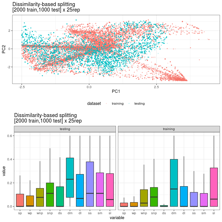
Figure 1. A 2D projection of two different datasets considering the first 2 principal components. In addition, the figure includes the boxplot distribution for each predictor variable in both datasets.
The Statistical Approach.
Answering the question whether two samples have the same distribution is a task that can be resolved applying statistical tests. The common tests used for comparing two distribution are chi squared for categorical variables and Kolmogorov-Smirnov (K-S) for numerical variables.
For a multiple variable dataset, the approach is quite simple: for each variable from the sample you should compare its probability distribution with the probability distribution of the same variable of the population. The result of the K-S test can be used in conjunction with information about variables importance to take a final decision about the dataset.
This simple statistical framework is very useful for discovering possible problems in your models when testing and training sets have some differences. Do not forget to check the assumptions for each statistical test and please remember this is just a tool that can provide you with some insights about possible problems in your data. Nothing more and nothing less. ⚠️Please use with caution ⚠️.
For more complete posts about this approach you can check here and also here
Finally, you can check other distance measures between two histograms here
The Algoritmic Approach
When projecting many predictors into two dimensions such as the case of PCA, intricate predictor relationships could mask regions within the predictor space where the model will inadequately predict new samples. As an alternative you can try the algorithmic described by Hastie et al. to get more detailed information about the similarities between two datasets. The general idea is to create a new dataset randomly permuting the predictors from the training set and then, row-wise concatenate to the original dataset set labeling original and permuted samples. You should check categorical variables was not permuted with a numerical one. Also is a good idea to apply some sort of normalization to the dataset before permuting the variables. Then, a classification model is run on the resulting dataset to predict the probability of new data being in the class of the original set. The benefit of this algorithmic approach is that easy to obtain an error number between the two datasets considered.
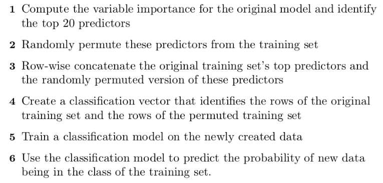
Figure 2. Pseudo code of the algorithm for building a model to get probability of a new data point is being similar of a given dataset. Taken from Max Khun’s Applied Predictive modeling book
Below is a simple R implementation I provide you as-is 😉
library(randomForest)
library(tidyr)
library(dplyr)

efron_simil<-function(train,prec_len){
  train<-train %>% select(1:prec_len)
  predictor_order<-sample(1:prec_len,prec_len)
  train_permuted<-train[,predictor_order]
  names(train_permuted)<-names(train)
  train_permuted$dataset<- "random"
  train$dataset<- "original"
  train<-rbind(train_permuted,train)
  train_model<-randomForest::randomForest(x=train[,1:10],
  y=as.factor(train$dataset))
}

calculate_efron_simil <- function(df_train, df_test,class) {
  results <- list()
  for (i in 1:25) {
    train <- df_train[[i]]
    test <- df_test[[i]]
    model <- efron_simil(train,ncol(train %>% select(-class)))
    predictions_prob <- predict(model, test, type = "prob")
    predictions <- ifelse(predictions_prob[,2]>0.5,"random","original")
    results <-
      rbind(
        results,
        table(predictions) %>% as.data.frame() %>%
          tibble::add_column(repetition =   i)
      )
  }
  results %>% tidyr::pivot_wider(names_from = predictions,
  values_from = Freq) %>%
    mutate(err = 1-(original / (original + random))) %>% select(err) %>%
    mutate(mean = mean(err), sd = sd(err))
}