
Inference with Observational Data
Disclaimer I’m far from being a statistician (Remember I’m just and old geek who forgot how to code), so the following text could be somewhat incorrect.
Recently at LABSIN, we were exposed to a dataset containing information about eye surgeries. The same technique was applied to a number of patients. However the dataset was not the result of a controlled experiment. In other words, there was no control over the different random variables in the dataset (lens type, Gender, age, etc). In particular there was a categorical variable with only two possible outcomes that showed a very unusual proportion according to state of the art. We wanted to do some inference: Were these results significant or we were fooled by the data? Also important it was to estimate the variability or precision of the observed proportion.
To sum up, we were asked about whether it was possible to say something beyond the observed results and this kind of request was a little different from the kind we use to received (mostly because our computer Science background).
A (slightly more) Formal Problem definition
There is one variable \(X\) with two possible outcomes \(X \in \{0,1\}\). And after sampling \(n\) from the population, we found that \(p\) of the times \(X=1\)
We have one observation of \(p\), as the result of carrying out a single sample of data. We now wish to infer about the future. We would like to know how reliable our observation of \(p\) is without further sampling.
Binomial model
The problem can be modeled using a Binomial distribution. The binomial distribution is frequently used to model the number of successes (\(p\)) in a sample of size \(n\) drawn with replacement from a population of size \(N\). In other words, it can be thought of as simply the probability of a SUCCESS or FAILURE outcome in an experiment that is repeated multiple times. In our case, we are going to consider each eye surgery as an independent experiment.
So for our particular sample, we can say that From 45 observed surgeries only 5 show an outcome=0 and the rest outcome=1.
Can we get an idea of the variability of such proportion?
Estimating the variability or precision of the proportion.
One proportion z-test
Since our random variable \(X\) follows a binomial distribution we can estimate the ‘margin of error’ or to use the proper term, confidence interval for the observed \(p\) using a one-proportion z-test. Under a one-proportion \(z\)-test, the binomial distribution is approximated to a normal distribution (see Figure 1), then we can use this approximation to estimate the confidence intervals.
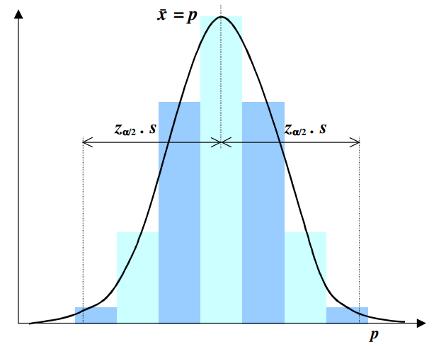
Figure 1. The Normal approximation to the Binomial plotted within the probabilistic range p ∈ [0, 1].
We only need to obtain \(\mu\) (expected value for \(p\)) and standard deviation \(\sigma\) and then calculate the confidence intervals for a given \(\alpha\) (the probability of rejecting the null hypothesis when it is true) using the \(z\) statistic.
\[ z=\frac{\mu-p}{\sigma} \]
In R we can use the function prop.test() that implements the Z test for proportions using Wilson’s ideas about approximating a binomial to normal distribution.
n<-45 # the total number of surgeries (trials)
p<-40 # the number of surgeries where outcome 1 was observed.
mu<-0.1 # the expected probability for observing outcome 1.

prop.test(p,n,mu,correct = FALSE, alternative = "two.sided")
## Warning in prop.test(p, n, mu, correct = FALSE, alternative = "two.sided"): Chi-
## squared approximation may be incorrect##
## 1-sample proportions test without continuity correction
##
## data: p out of n, null probability mu
## X-squared = 311.17, df = 1, p-value < 2.2e-16
## alternative hypothesis: true p is not equal to 0.1
## 95 percent confidence interval:
## 0.7650090 0.9515953
## sample estimates:
## p
## 0.8888889So according to the one-proportion \(z\)-test results, we can say that surgeries observing an outcome=1 will be between 76% and 95% of the times (with 95% confidence level) In other words, if someone repeats this process (i.e. it takes another sample from the population of eyes surgeries using the same technique), there will be 95% of chance that 75 to 96 percent of the surgeries have outcome=1.
The \(z\)-test for proportions provides us not only with information about confidence interval but also let us to test different hypothesis. For instance, in the above example we are testing that on average the outcome will be observed 10% of the times. So the null hypothesis is \(H_{0}=0.1\) and the alternative hypothesis is \(H_{A}!=0.1\). According to z-test p-value we can reject the null hypothesis. In other words, if someone else samples another eye surgeries using the same technique, there is 95% chance of not observing the outcome 10% of the time.
Notice that most of the time we would check if there were 30 data points or more, but for a proportion, we do something slightly different. When data is binary, like we have here, the central limit theorem kicks in slower than usual. The standard thing to check is whether:
\[n.(p/n)>5 \]
\[n.(1−p/n)>5\]
So if we do:
\[ 45 . (40/45) ~= 40 \]
\[ 45 . (1-(40/45)) ~= 5\]
Oops, we have a problem… Actually if we look carefully at prop.test() output we can see a Warning message saying something like Chi-squared approximation may be incorrect So, what we can do?
The exact binomial test
So far we have employed the Normal approximation to the Binomial distribution. However, it is possible to use an binomial exact test.
This test should be the standard against which other test statistics are judged. The significance level and power are computed by enumerating the possible values of \(p\), computing the probability of each value, and then computing the corresponding value of the test statistic. In R we can use the function binom.test() that implements the exact binomial test using Clopper & Pearson ideas.
n<-45 # the total number of surgeries (trials)
p<-40 # the number of surgeries where outcome 1 was observed.
mu<-0.1 # the expected probability for observing outcome 1.

binom.test(p,n,mu, alternative = "two.sided")
##
## Exact binomial test
##
## data: p and n
## number of successes = 40, number of trials = 45, p-value < 2.2e-16
## alternative hypothesis: true probability of success is not equal to 0.1
## 95 percent confidence interval:
## 0.7594642 0.9629233
## sample estimates:
## probability of success
## 0.8888889The binomial exact test reports that surgeries observing outcome 1 will be between 76% and 96% of the times (with 95% confidence level) here is a difference in the confidence interval got by the one-proportion z-tes and no error was reporter in this case.
Conclusions
Despite the information and selection bias are a major obstacle to drawing valid conclusions from an observational study, it is still possible to do inference from observational data. If we apply a binomial model there are several methods to analyze the observed proportion, although these legacy (such as one-proportion z-test) methods are still presented in textbooks, their power and accuracy should be compared against modern exact method before they are adopted for serious research.
References
[1] A vignette about Z-test for proportions in R.
[2] “Analysis of Observational Studies: A Guide to Understanding Statistical Methods”. A recommended article about dealing with Observational data. Most of the ideas of this post were stolen from here. 😉
[3] “Binomial confidence intervals and contingency tests: mathematical fundamentals and the evaluation of alternative methods.” Another good article discussing the math behind Binomial and Z-test proportional tests.
[4] Binomial distribution assumptions.
[5] A very nice article discussing the confidence interval for proportions. Very similar (but more complete) to this post.