
How confident is Random Forest about its predictions?
The problem is quite simple: you have collected a good tabular dataset. After cleaning and doing the usual Machine Learning procedure, you decide to try the good ol’ Random Forest from our friend Leo. You train the model and test it on unseen data and surprisingly you got some very decent results.
But now, you asked yourself: given a prediction on a particular example, how sure is Random Forest about it. Or if you put it in different words: if we change the training dataset just a little bit, will Random Forest give you the same result for that particular example?
You should notice this question is a little different from the usual Machine learning issue regarding model future performance estimation. The traditional question is more focused on how different will be the overall performance of a given model if we use a different dataset. (read about average generalization error here). Despite their similarities, the key here is the word overall. We are not interested in the overall performance, but in a particular example in our test dataset. For dealing with the former, you will use approaches such as K-fold cross-validation or the classic Monte Carlo split. For the latter, there are several approaches, but clearly, the term Confidence interval (CI) arises as a possible solution.
Q: Given a prediction on a particular example, how sure is Random Forest about it?
Confidence intervals
Since Random Forest (RF) outputs an estimation of the class probability, it is possible to calculate confidence intervals. Confidence intervals will provide you with a possible ‘margin of error’ of the output probability class. So, let’s say RF output for a given example is 0.60. The usual approach is to assign that example to the positive class (>0.5). But, what would happen if you obtain a confidence interval of 0.15. That means that the probability range will lay between 0.45 and 0.65 (with a certain alpha level). And consequently, RF has effectively abandoned any hope of unambiguously classifying the example. On the other hand, for a CI value of 0.05 then, the probability range will lay between 0.55 and 0.65, and under such a scenario, the classification will be always positive for that given example. To sum up, the lower the CI the more confident you will be about RF predictions.
A practical example
Let’s try an example using a dataset containing information about malicious and normal network traffic connections.
You do the usual 70/30 split in train and test sets and then you train four different models using Random Forest varying the number of trees (aka estimators). In the end, you get the following table:
| Number of Trees | Accuracy | Sensitivity | Specificity |
|---|---|---|---|
| 50 | 0.969 | 0.990 | 0.720 |
| 100 | 0.960 | 0.986 | 0.655 |
| 500 | 0.964 | 0.987 | 0.702 |
| 1000 | 0.969 | 0.987 | 0.703 |
The problem here (notice it is oversimplified) is which model you will choose. Accuracy and Sensitivity are practically the same. And even for specificity you have all but the model with 100 trees showing the same values. If you follow a traditional policy of selecting the best value. Then, RF with the number of trees = 50 will be the choice model. However, if you look at the CI distribution for each of the output probabilities, things could be different.
Figure 1. shows a plot of test-set predictions against estimates of standard error (\(se\)) for all four RF models. Orange dots refer to instances incorrectly classified while blue to correctly classified. The solid curves are smoothing splines that fit through the data. Remember that \(CI = mean\pm se\) .
Now, you can see some observable differences between the four RF models. The model using 50 trees has a very large \(se\) values, in some cases very close to 1. So it basically means that the model is not sure about anything and the results from Table 1 should not be taken so seriously. Moreover, It is possible that the model is overfitting the data. On the other hand, the model using 1000 trees and all \(se\) values under 0.25, it is certainly more confident about its predictions.
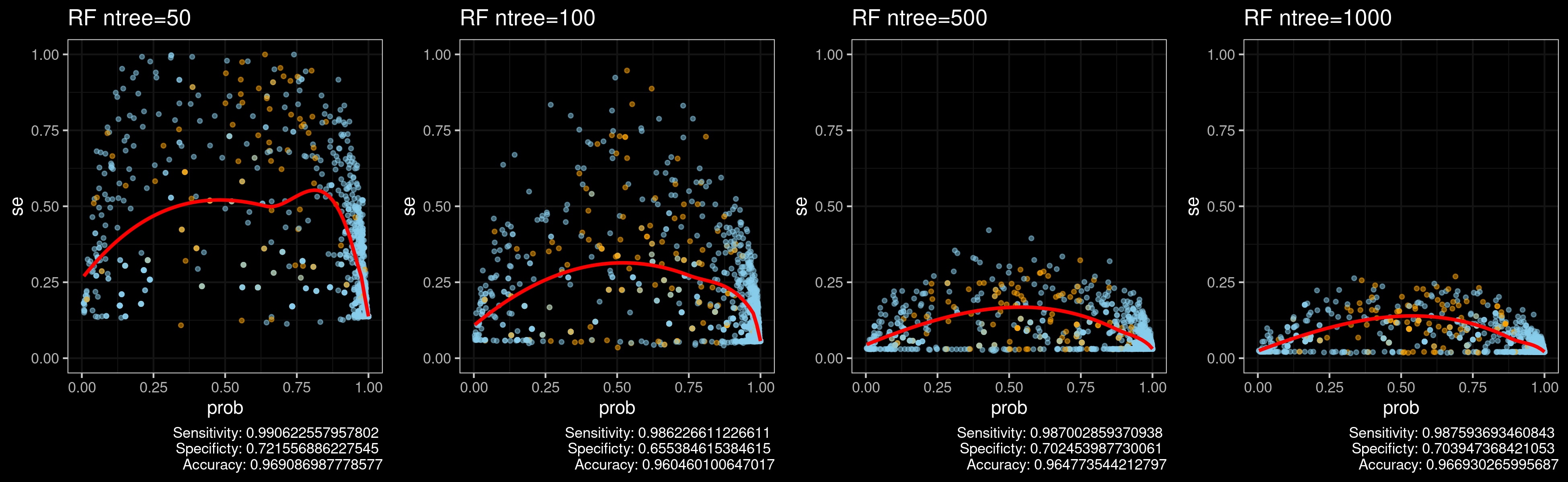
Figure 1. Predictions against estimates of standard error ($se$) for all four RF models.
Notice the results in Figure 1 are consistent with the way RF works for binary classification problems. If you use more trees, you are reducing the variance of the of de model and the RF will be more confident with its own predictions. An intuition about this is given in this article. The article states that for each sample, the ensemble will tend toward a particular mean prediction value for that sample as the number of trees tends towards infinity.
Under the hood
So, how is CI calculated for random forests?, there are several approaches (see the list of papers at the end of the post). But the one I used for the above example is based on the article Confidence Intervals for Random Forests: The Jackknife and the Infinitesimal Jackknife (Wager, Hastie and Efron 2014)
The wager approach uses the Jackknife resampling technique for estimating the CI. Jackknife was proposed by John Tukey in 1956. The general idea behind Jackknife is that a parameter estimate can be found by estimating the parameter for each subsample omitting the i-th observation.
More formally, you have to generate a jackknife sample that has the value \(x_i\) removed and then compute the i-th partial estimate of the statistic using this sample,
\[ \hat{\theta_{i}}(x_1,...,x_{x-1},x_n) \]
We then turn this i-th partial estimate into the i-th pseudo value \(\hat{\theta}_{i}*\) using the following equation
\[ \hat{\theta}_{i}*=n\hat{\theta} - (n -1) \hat{\theta}_{i} \]
where \(\hat{\theta}\) is the estimate using the full dataset. The previous equation is the bias-corrected jackknife estimate.
Let’s see an example in R. We have a vector \(x\) and we define the function tetha that corresponds to the coefficient of variation (i.e. the statistics we want to estimate)
x <-c(8.26, 6.33, 10.4, 5.27, 5.35, 5.61, 6.12, 6.19, 5.2,
7.01, 8.74, 7.78, 7.02, 6, 6.5, 5.8, 5.12, 7.41, 6.52, 6.21,
12.28, 5.6, 5.38, 6.6, 8.74)

theta <- function(x) sqrt(var(x))/mean(x)
We create two vectors, jack and pseudo and we need to fill in the elements of the jack sample vector as follows. For \(j<i\), the \(j − 1\)th element of jack is the d th element of x. We can state all this using a logical if .. else statement within afor loop,
jack <- numeric(length(x)-1)
pseudo <- numeric(length(x))

# creates datasets with all but the ith sample
for (i in 1:length(x)) {
  for (j in 1:length(x)) {
    if(j < i) jack[j] <- x[j]
      else if(j > i) jack[j-1] <- x[j]
  }
  # calculate the estimate for ith
  pseudo[i] <- length(x)*theta(x) -(length(x)-1)*theta(jack)
}
Now we can calculate approximate 95% confidence interval by calculating the upper and lower limits
mean(pseudo) + qt(0.975,length(x)-1)*sqrt(var(pseudo)/length(x))## [1] 0.3729806mean(pseudo) - qt(0.975,length(x)-1)*sqrt(var(pseudo)/length(x))## [1] 0.1504947Giving the approximate 95% jackknife confidence interval as 0.150 to 0.372. Please note that this is an oversimplified explanation of the jackknife technique. The method described in Wager’s article is clearly more advanced, but I think this could help you (and me) to understand the basics of the approach.
Some final words…
The Jackknife method like any other resampling method is computationally expensive and could be difficult to apply to the large datasets used nowadays.
Please keep in mind that here you are not dealing with prediction intervals (i.e., intervals that cover new observations \(Y_{i}\) with high probability), instead, you are dealing with confidence intervals (i.e., intervals that cover \(\mu(x) = E[Y|X=x]\) with high probability. In case you need the former, using Quantile regression approaches seems to be the way to go.
References
[1] The ranger package for R is a fast implementation of Random forest that includes the Wager’s approach for confidence intervals.
[2] Quantile Regression Forests provides a method for prediction intervals.
[3] The U-statistics approach of Mentch and Hooker (2006) is another approach for confidence intervals.
[4] A discussion about implementation details is available on Github.
[5] Professor Chen has some notes discussing the basics of several resampling methods using for estimating statistics. I stole my example from him.
[6] A reproducible example using ranger package for SE calculation.
[7] Prof. Hyndman disscues the differences between Confidence and Prediction Intervals.