Tackling the limitations of tree-based algorithms

Recognizing the problem

OK, but what are the implications of this limitation?. Let’s see the problem in action. First we are going to generate a training set and a test with only one predictor variable.

library(dplyr)
set.seed(19091973)
x1<-rnorm(50,30,30)
error<-rnorm(50,30,30)
y1<-(4*x1)+error

x1_test<-rnorm(50,160,30)
error<-rnorm(50,30,30)
y1_test<-(4*x1_test)+error

sample_train<- data.frame(dataset="training",y=y1,x=x1)
sample_test<-  data.frame(dataset="testing",y=y1_test,x=x1_test)

In this particular dataset, the range of predictor values use for training does not overlap with values from the testing dataset. Let’s plot the data to see what am I talking about.

library(ggplot2)
rbind(sample_train,sample_test)  %>% ggplot()+
  geom_point(aes(x=x,y=y,color=dataset),shape=21)+
  ggdark::dark_theme_bw()+
  labs(title="Simulated data for regression",
  subtitle = "Datasets with different range values for predictor variable")+
  guides(color=guide_legend(title="Dataset"))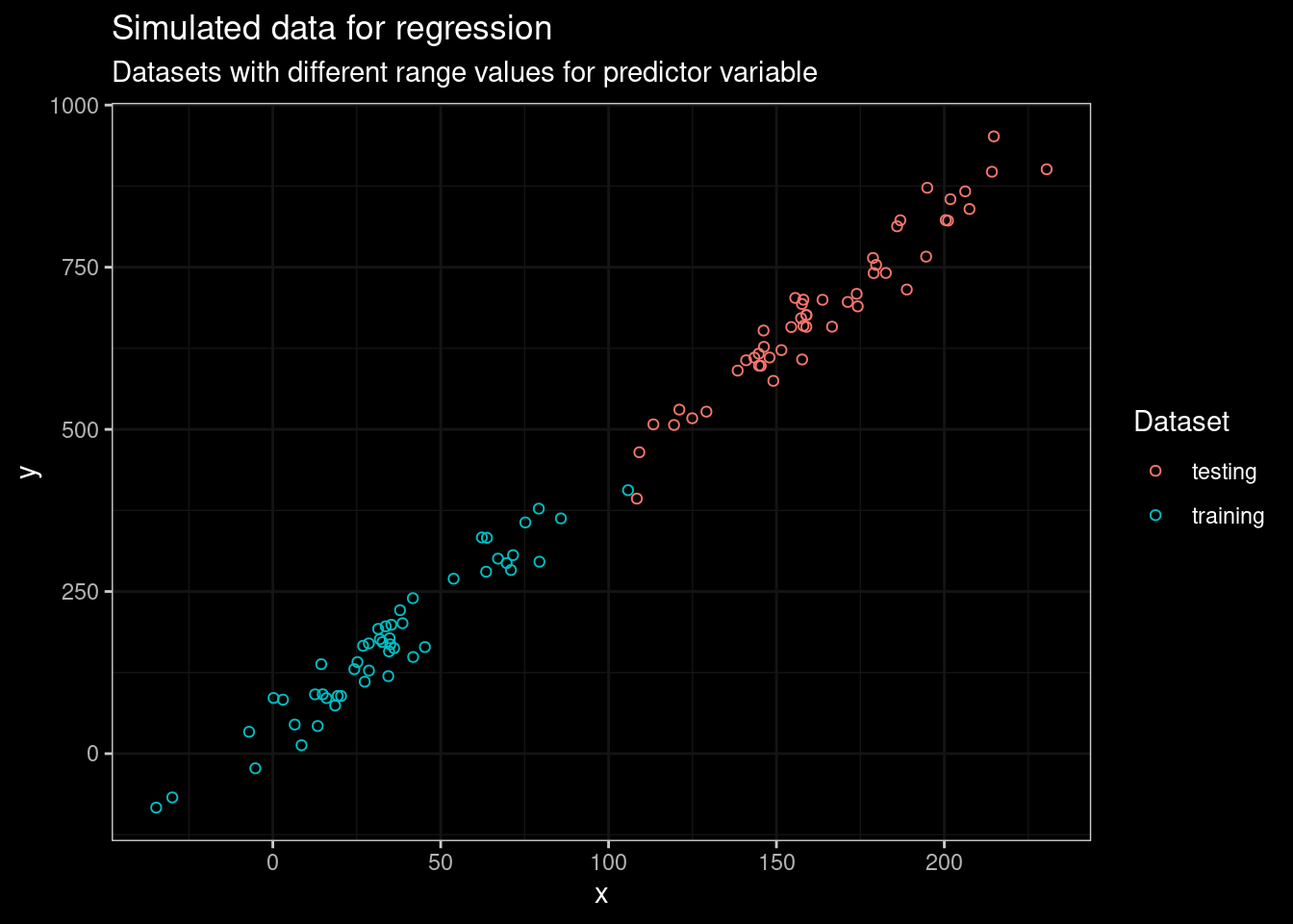

Figure 1: Plot of simulated data for testing and training models

There’s a remarkable linear trend in the training dataset, and the tendency continues in the testing dataset. The regression problem can easily be handled by fitting a linear model. Let’s verify this with the following code.

First, a simple function for include predictions from a given model into a dataframe.

# A helper function for facilitating ploting data
create_predictions_df <- function(model, train, test){

  if (class(model) == "catboost.Model"){
    test_pool<-catboost.load_pool(test %>% select(-dataset,-y), 
                              label = test$y)
    test_predictions<-catboost.predict(model,test_pool)
    train_pool<-catboost.load_pool(train %>% select(-dataset,-y), 
                              label = train$y)
    train_predictions<-catboost.predict(model,train_pool)
  } else {
    test_predictions <- predict(model, test %>% select(-dataset,-y))
    train_predictions <- predict(model, train %>% select(-dataset,-y))
  }
  
  predictions_test_df <- 
    data.frame(dataset = "test", y = test$y, x = test$x, predictions =
                 if(class(model) == "ranger" || "grf" %in% class(model))  
                    test_predictions$predictions else 
                    test_predictions)
  predictions_train_df <- 
    data.frame(dataset = "train", y = train$y, x = train$x, predictions =
                 if(class(model) == "ranger" || "grf" %in% class(model))  
                    train_predictions$predictions else 
                    train_predictions)
 rbind(predictions_train_df,predictions_test_df)
}

Then, we train a simple linear regression model using training data and try to predict the outcome for testing.

# Fit a linear model
lm_fit<-lm(y~x,data=sample_train %>% select(-dataset))

create_predictions_df(lm_fit,sample_train,sample_test) %>%
  ggplot()+
  geom_line(aes(x=x,y=predictions),color='orange')+
  ylab("y")+
  geom_point(aes(x=x,y=y,color=dataset),shape=21)+
  ggdark::dark_theme_bw()+
  labs(title="Linear Regressor",
  subtitle = "Datasets with different range values for predictor variable")+
  guides(color=guide_legend(title="Dataset"))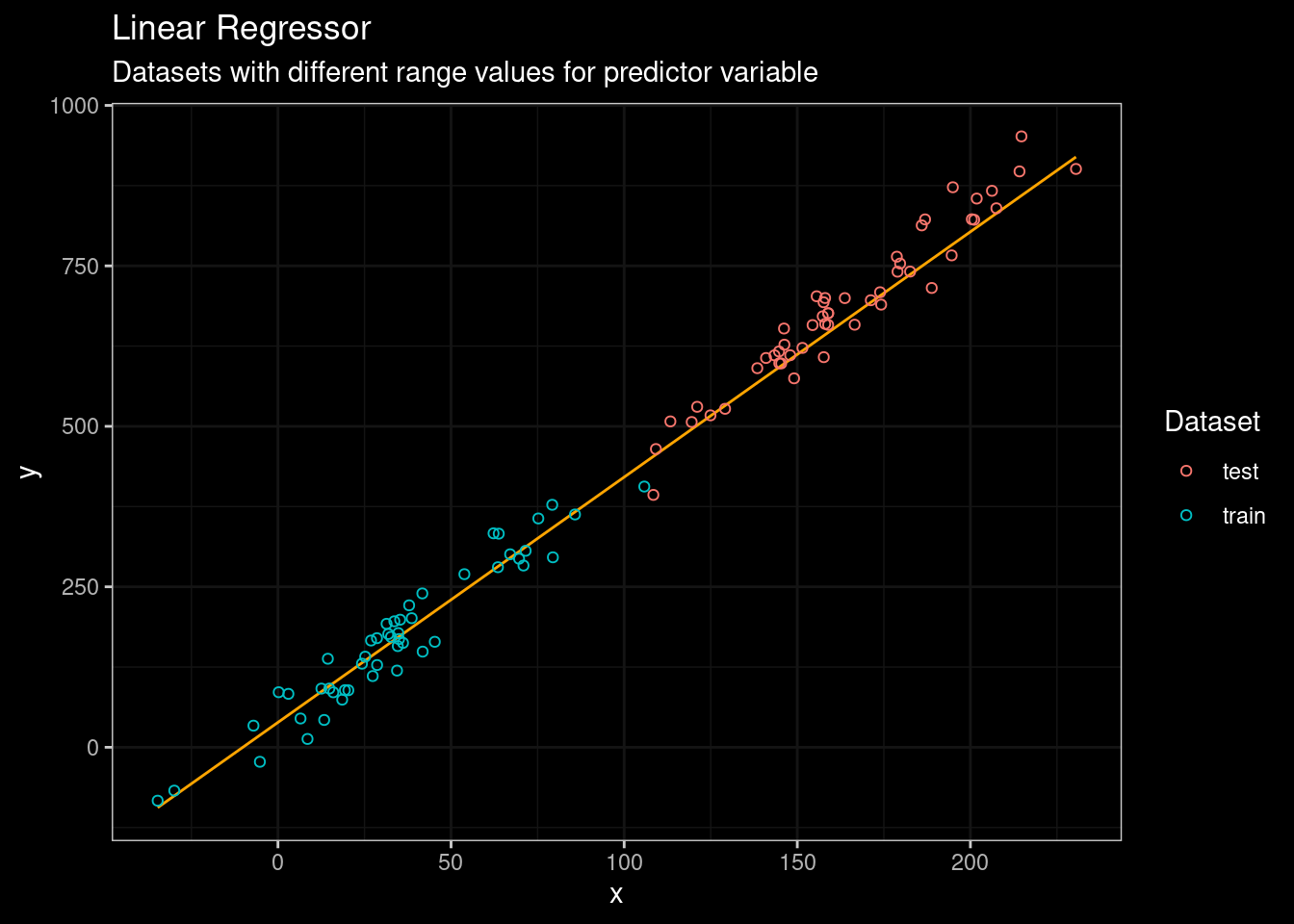

Figure 2: Linear Regression results

No problem man! As expected the linear regressor model did a pretty decent work fitting the data (see orange line). Now, let’s start with a classic tree-based (CART) approach. I will use the rpart package.

library(rpart)
part_fit<-rpart(y ~ x,data = sample_train,control = rpart.control(cp = 0.001))

create_predictions_df(part_fit,sample_train,sample_test)  %>%
  ggplot()+
  geom_line(aes(x=x,y=predictions),color='orange')+
  geom_point(aes(x=x,y=y,color=dataset),shape=21)+
  ylab("y")+
  ggdark::dark_theme_bw()+
  labs(title="Tree Regressor",
  subtitle = "Datasets with different range values for predictor variable")+
  guides(color=guide_legend(title="Dataset"))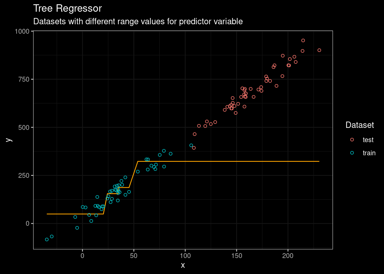

Figure 3: CART results

Boooh! . We can see that rpart model was unable to predict the outcome on the testing set. But, CART are not the state of the art of tree-based algorithm. So let’s try the good ol’ Random Forest algorithm. In this particular case, I will use the ranger package, a fast and modern implementation of Random Forest (highly recommend if you prefer R).

library(ranger)
# Fit data on training set
rf_fit<-ranger(y ~ x, sample_train, num.trees = 100, keep.inbag = TRUE)

create_predictions_df(rf_fit,sample_train,sample_test)  %>%
  ggplot()+
  geom_line(aes(x=x,y=predictions),color='orange')+
  geom_point(aes(x=x,y=y,color=dataset),shape=21)+
  ylab("y")+
  ggdark::dark_theme_bw()+
  labs(title="Random Forest Regressor",
  subtitle = "Datasets with different range values for predictor variable")+
  guides(color=guide_legend(title="Dataset"))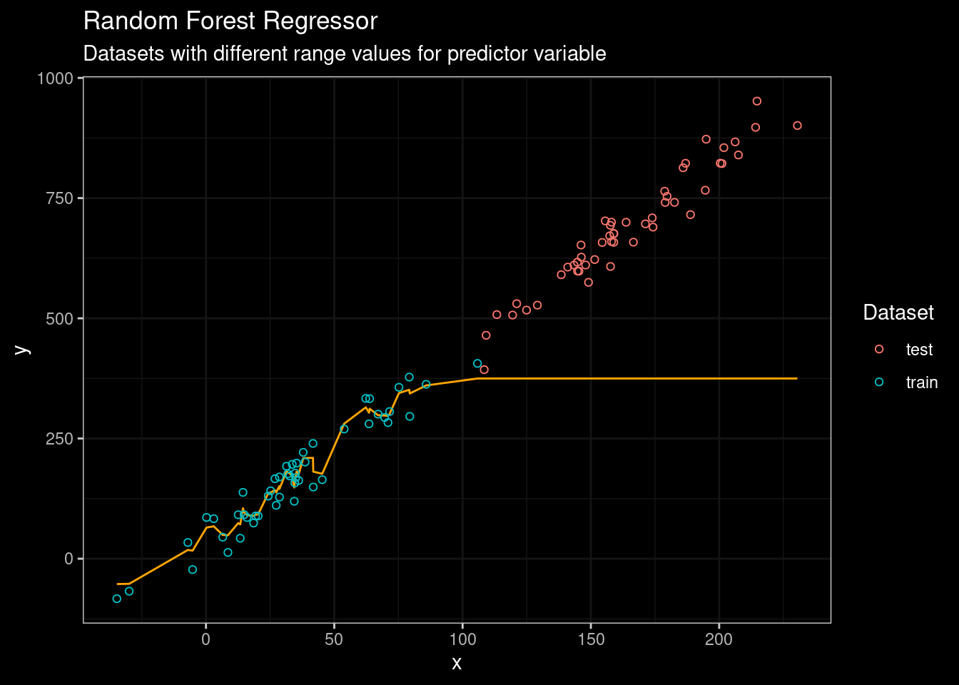

Figure 4: Random Forest results

Random Forest did a very good job fitting the data from the training set. However, its performance on testing data was really embarrassing. No way man! 😥 😥. What about a state-of-the-art tree-based algorithm such as catboost? Let’s see.

library(catboost)
# Fit data on training set
train_pool<-catboost.load_pool(sample_train %>% select(-dataset,-y),
                               label = sample_train$y)
cat_fit<-catboost.train(train_pool)

create_predictions_df(cat_fit,sample_train,sample_test)  %>%
  ggplot()+
  geom_line(aes(x=x,y=predictions),color='orange')+
  geom_point(aes(x=x,y=y,color=dataset),shape=21)+
  ylab("y")+
  ggdark::dark_theme_bw()+
  labs(title="Catboost Regressor",
  subtitle = "Datasets with different range values for predictor variable")+
  guides(color=guide_legend(title="Dataset"))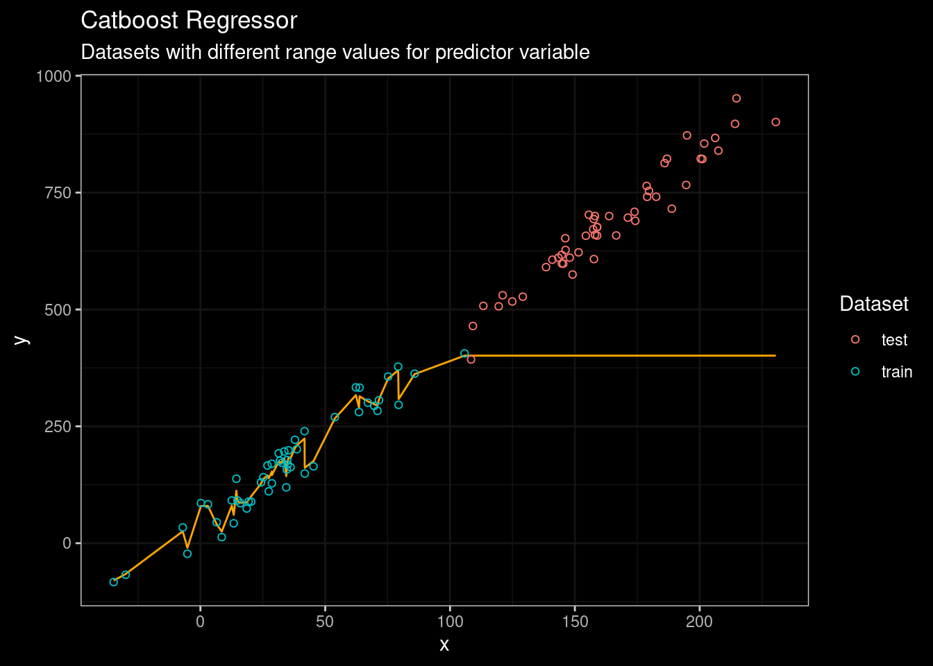

Figure 5: Catboost results

Mmmmm… not a big difference compared with Random Forest. Well, the problem is pretty obvious. When Random Forest, CART, or catboost are used for regression the output for a leaf equals the average of the data points belonging to the leaf. Moreover, the threshold used for splitting the data is also calculated from the average of the observed data points. Look at the resulting tree when rpart is used..

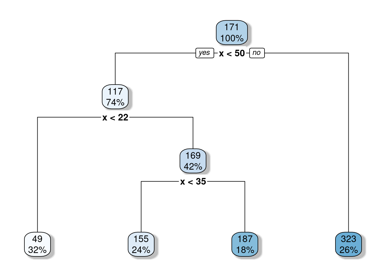
Figure 6: Resulting CART for training data.

The threshold value of the root node is set to 171. Any value for the predictor variable ( x ) greater than 171 will end in the right leaf and the average outcome ( y ) value for those observations with ( x > 171 ) equals 323. So, it means that the predicted outcome will be bound at 323. And in fact, we can confirm that if we look again at Figure 3.

Most of Tree-based algorithms are bound by the average values coming from observations used in training. .

Tackling the problem.

Fortunately, very smart people have noticed the issue a long time ago, and provide us with some alternatives to deal with this limitation of tree-based algorithms. But keep in mind these alternatives, do not provide us with a concluding solution, just some minor improvements to the original problem.

Quinlan’s M5 model tree

One of the first approaches was developed by the legendary Ross Quinlan (the father of the C4.5 algorithm). In the article Learning with continuous classes, Quinlan developed the idea of building a linear regression function using the data points observations belonging to that leaf instead of the average. The resulting algorithm named M5, constructs tree-based piecewise linear models. Max Khun has developed the Cubist R package that implements similar ideas.

library(Cubist)
# Fit data on training set
m5_fit<-cubist(x=sample_train %>% select(-dataset,-y), y=sample_train$y)

create_predictions_df(m5_fit,sample_train,sample_test)  %>%
  ggplot()+
  geom_line(aes(x=x,y=predictions),color='orange')+
  geom_point(aes(x=x,y=predictions),color='orange',shape=21,size=0.5)+
  geom_point(aes(x=x,y=y,color=dataset),shape=21)+
  ylab("y")+
  ggdark::dark_theme_bw()+
  labs(title="M5 Regressor",
  subtitle = "Datasets with different range values for predictor variable")+
  guides(color=guide_legend(title="Dataset"))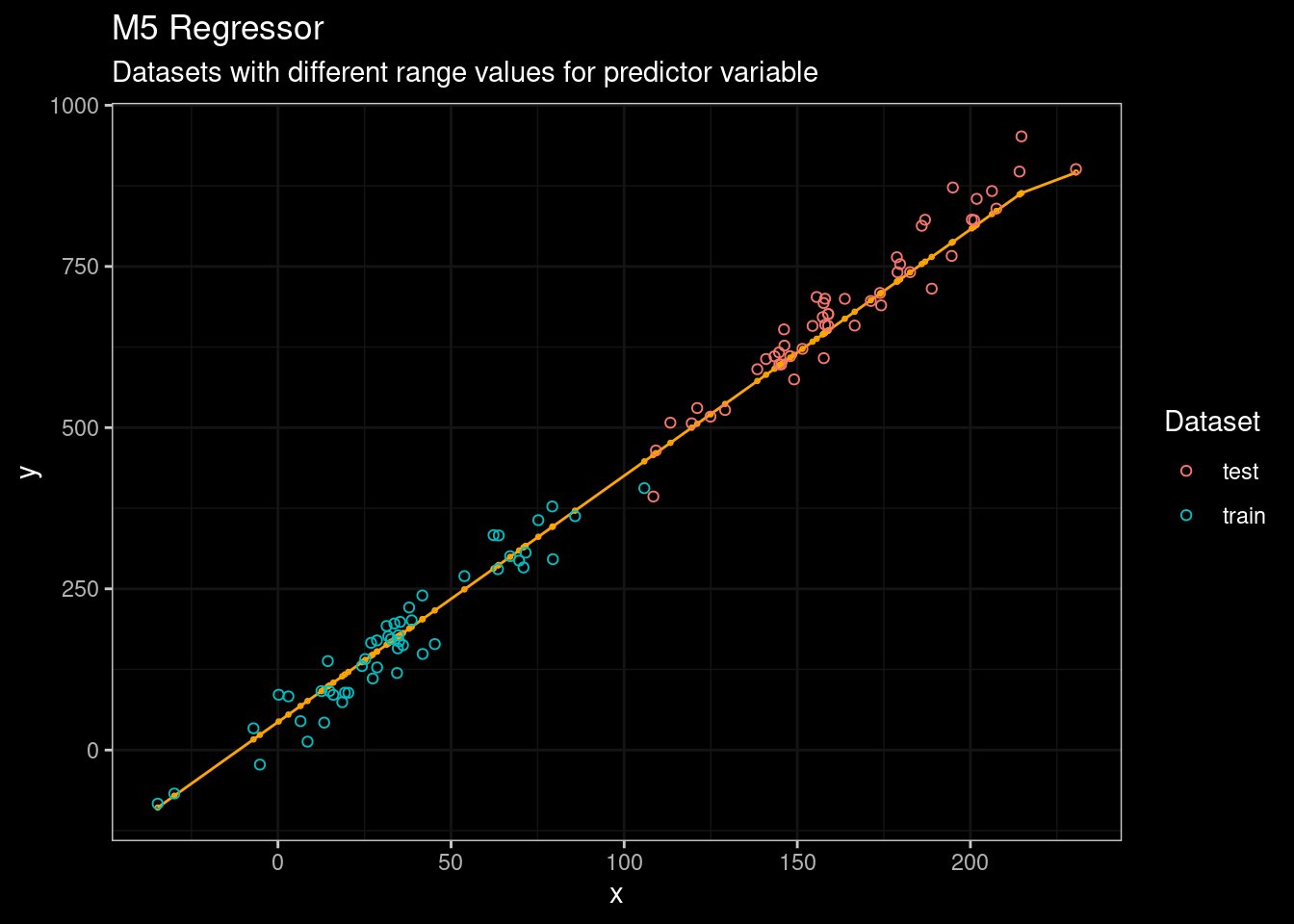

Figure 7: M5 results

Not bad for an algorithm from 1992 💪. In addition, the Cubist package also includes the idea of committees, a boosting-like scheme called where iterative model trees are created in sequence. Unlike traditional boosting, stage weights for each committee are not used to average the predictions from each model tree; the final prediction is a simple average of the predictions from each model tree.

Linear Local Forests

People from Stanford led by Stefan Wager (see my post about RF confidence interval) have come up with the so-called Linear Local Forest, which is actually very similar to the M5 approach. The idea is to instead of using the weights to fit a local average, they use them to fit a local linear regression, with a ridge penalty for regularization (see paper here). The authors have provided us with the grf package which implements the LLF approach in addition to several other extensions to random forest.

library(grf)
set.seed(1920202)
grf_fit<-ll_regression_forest(X=sample_train %>%
                                select(-dataset,-y) %>% as.matrix(), 
                              Y=sample_train$y, num.trees = 2000)

create_predictions_df(grf_fit,sample_train,sample_test)  %>%
  ggplot()+
  geom_line(aes(x=x,y=predictions),color='orange')+
  geom_point(aes(x=x,y=y,color=dataset),shape=21)+
  ylab("y")+
  ggdark::dark_theme_bw()+
  labs(title="Linear Local Forest Regressor",
  subtitle = "Datasets with different range values for predictor variable")+
  guides(color=guide_legend(title="Dataset"))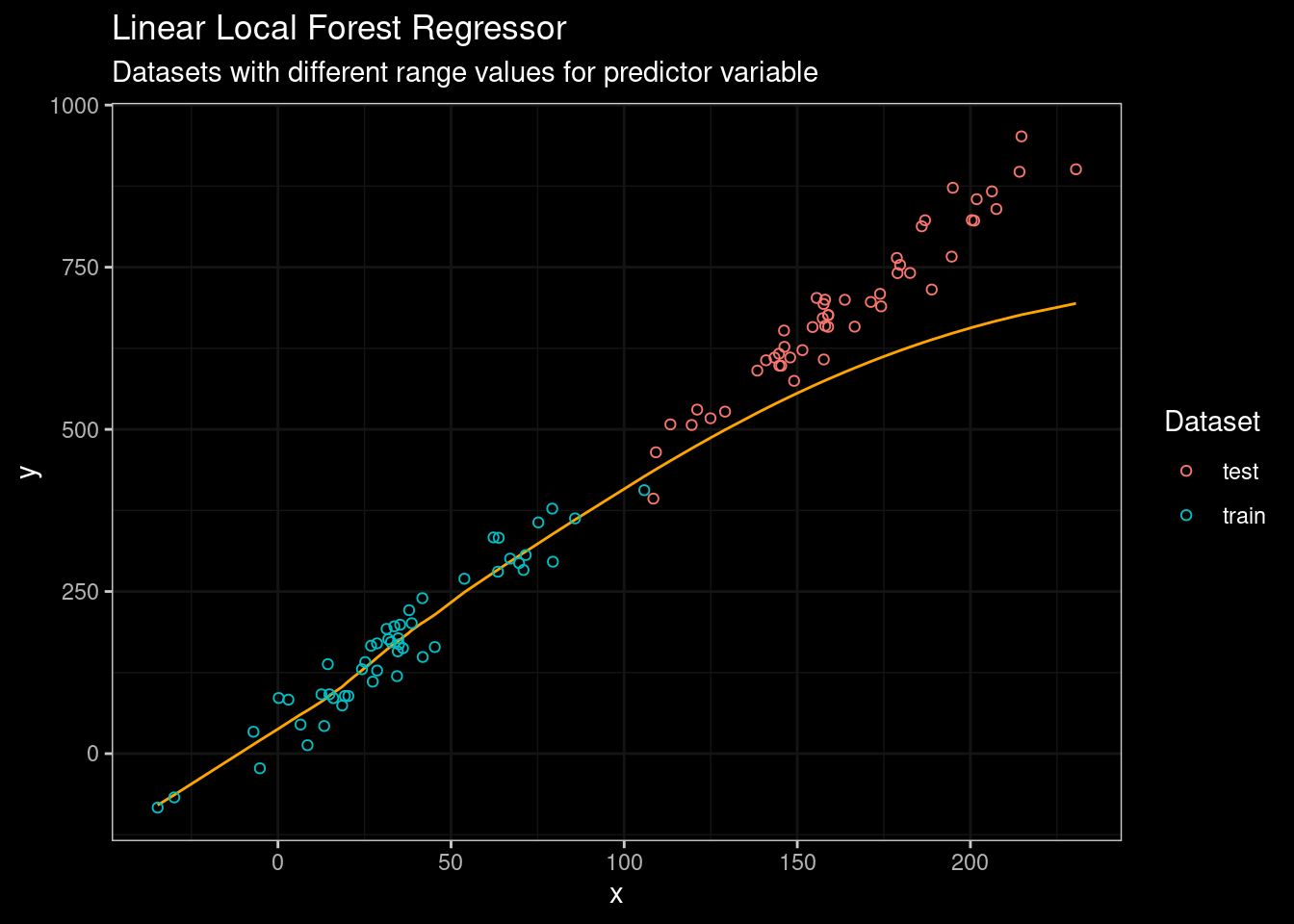

Figure 8: LLF Results

Well, this is definitively better. However, despite LLF is performing better than standard Random Forest, the truth is that LLF was not designed with extrapolation in mind. So their performance on other more complex datasets could not be the same as in the figure above

Just a few more words…

This post includes only toy examples for all the cases, certainly, we need to conduct a test on a more realistic dataset to get an idea of the real limitation of Random Forests and the actual benefits of the mentioned approaches. A clear conclusion is that Random Forests and other tree-based approaches are not always the way to go when dealing with regression problems. Moreover, If you’re interested in forecasting models, I’d suggest using other algorithms specifically designed for time-series data.

A similar situation arises in classification problems when new categories are observed during prediction. I’m not talking about outcome categories, but predictor categories. Random Forests and tree-based algorithms will be bound to observed categories (pretty obvious isn’t it) and when a new category arises, the algorithm will treat it as one of the already observed. It will be great if instead of choosing any arbitrary category value, the algorithm would be able of choosing the closest in terms of semantics. For now, the default option under these scenarios is to retrain the algorithm with new data…

More info here

[1] This post in Medium provides a much more detailed explanation of the limitation of Random Forest and the use of Regression Random Forest for tackling the issue.

[2] Learning with continuous classes by Ross Quinlan, an article discussing the M5 algorithm.

[3] A paper discussing a new approach called regression-enhanced random forests (RERFs).

[4] A medium post discussing a python implementation of regression-enhanced random forests (RERFs).

[5] Local Linear Forest, an approach from Stanford Group. (Arxiv paper.)

[6] GRF, an R package implementing Local Linear Forests.